a room
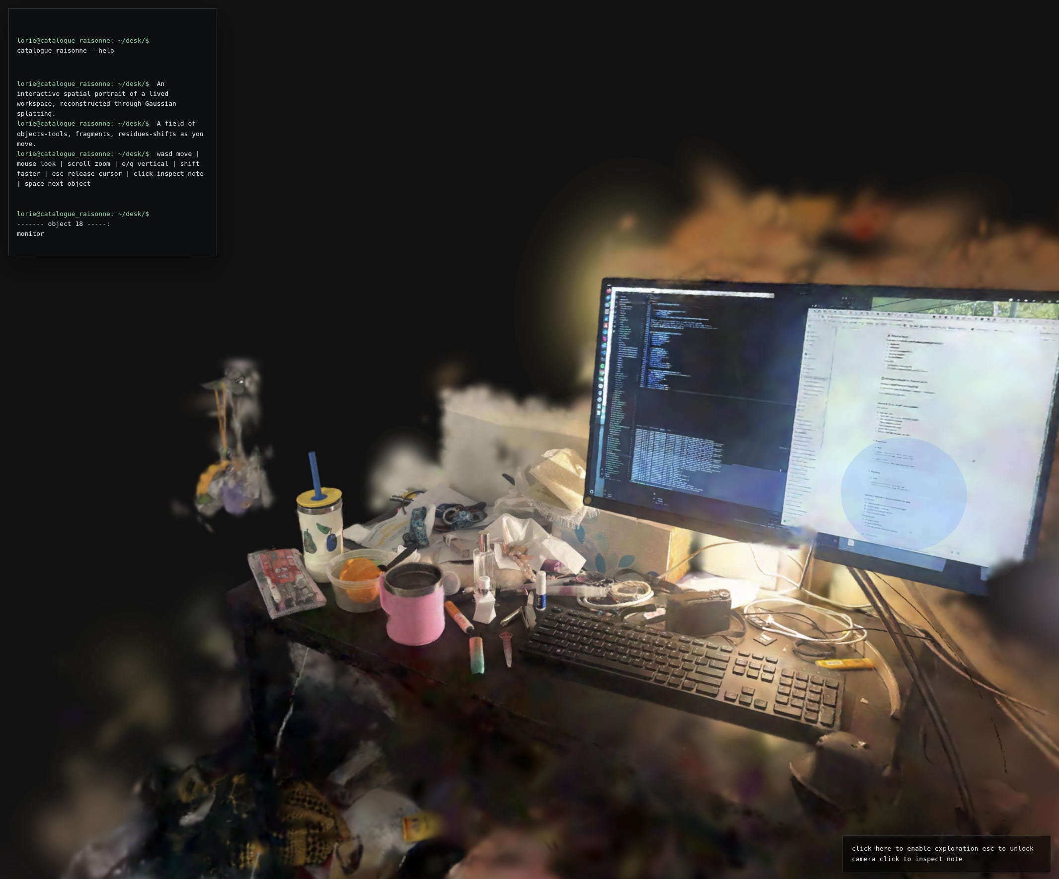
my work space annotated.

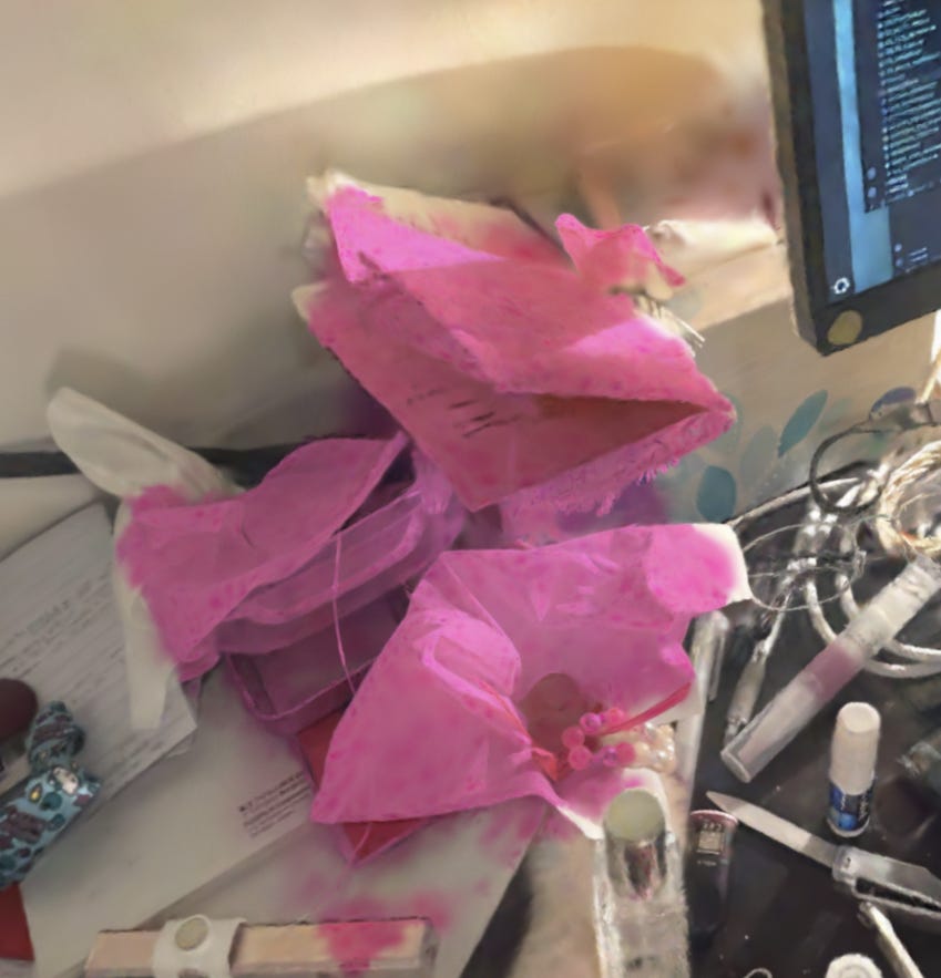
My studio and bedroom at Carnegie Mellon are not neutral spaces. They are sites where an education has physically reorganized my habits, the objects I keep, the way I arrange things on a desk. I wanted to capture them — not as photographs, not as architectural models, but as something navigable and interactive, where a viewer could move through the space and read it the way I’ve learned to read it: as evidence.
The technical path from that idea to a working demo turned out to be much messier than I expected. This is the process writeup. It includes the things that worked, the things that failed badly, and a probably unnecessary amount of detail about HDBSCAN clustering parameters.
Inspiration: the room as archive
Two artists kept coming up when I was thinking through what this project was actually doing. The first is Tracey Emin, whose My Bed (1998) turns an intimate domestic site into public evidence. The work doesn’t represent a bedroom — it presents one, unedited, as a record of emotional and bodily experience. What Emin establishes is that the arrangement of a lived space, its mess, its proximity structures, its traces of use, constitutes a form of autobiography that formal representation can’t achieve. The decision not to clean, not to curate, turns accumulation into argument.
The second is Gala Porras-Kim, whose practice interrogates how museums and archives classify and possess objects, especially when those objects exceed or resist the categories imposed on them. Her work asks what is lost when an artifact is labeled — what violence is embedded in the act of naming, and what forms of meaning survive only in the gaps between institutional categories.
These two concerns shaped the project from the start. Emin told me: don’t clean the room before you scan it. The mess is the point. Porras-Kim told me: be suspicious of the moment you start assigning labels. That suspicion ended up driving the most interesting technical choice in the pipeline — using CLIP not to classify objects into categories, but to query the space with deliberately non-taxonomic prompts like something that has been touched many times or an object that holds emptiness. More on that later.
The institutional question underneath all of this: how has Carnegie Mellon shaped not only what I make, but where and how I make it? The studio and bedroom became the sites where that question becomes visible — not through explicit narration, but through arrangement, accumulation, and use. Objects as evidence of a way of being formed.
Capture: what I tried and what actually worked
Attempt 1: COLMAP photogrammetry (did not work)
The original plan was standard photogrammetric reconstruction: take a few hundred photos of each room from overlapping viewpoints, run them through COLMAP to estimate camera poses and build a sparse point cloud, then train 3D Gaussian splats from that initialization.
COLMAP needs feature matches between images. In a bedroom, there is almost no good texture on large surfaces — walls are flat, the ceiling is flat, bed linens are flat. COLMAP kept failing to register most of my frames, producing sparse reconstructions that covered maybe 30% of the room with large gaps exactly where the interesting stuff was: the desk, the wall where my paintings hang, the corner with the cables and hard drives.
failure log
COLMAP feature matching failed to register ~60% of input images. The living-in-a-dorm-room problem: insufficient texture on large surface areas (walls, ceiling, bed), reflective surfaces on the monitor, and low-contrast regions near the window. The sparse point cloud that came out had a beautiful dense cluster of points on my houseplant and essentially nothing else useful. The 3DGS training initialized from this produced floating blobs in empty space and refused to converge anywhere near the desk.
I tried adjusting COLMAP’s feature matching parameters, forcing exhaustive matching instead of sequential, running on a downscaled version of the images. The sparse cloud got marginally better and then stopped improving. The fundamental problem was the scene itself: photogrammetry works poorly in environments designed to be lived in rather than scanned.
Attempt 2: Scaniverse SLAM (this worked)
I switched to Scaniverse, an iPhone app that uses LiDAR + visual SLAM (Simultaneous Localization and Mapping) to reconstruct scenes in real time. SLAM doesn’t depend on finding feature matches between static image pairs — it tracks the sensor pose continuously as you move, fusing depth from the LiDAR sensor with visual information from the camera. This makes it dramatically more robust in the low-texture environments that kill COLMAP.
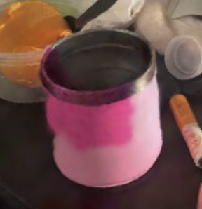
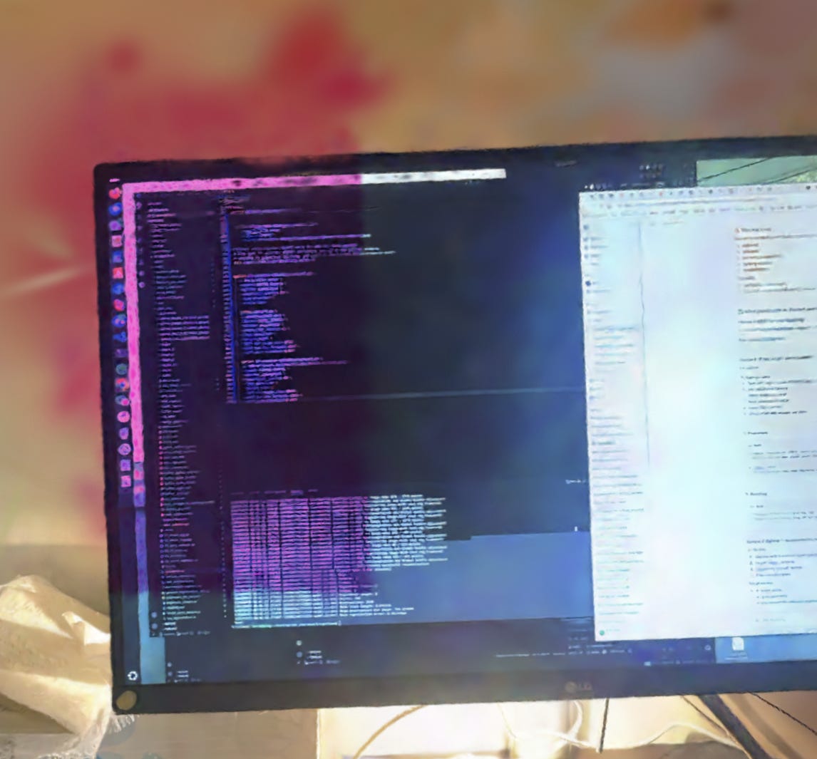
Scaniverse can export directly to Gaussian splats. The export quality isn’t as high as a carefully trained 3DGS from a clean COLMAP initialization — the splats are denser in some regions and sparse in others, and there are more floaters (more on those shortly). But it actually covers the whole room, which COLMAP could not. You can see the desk, the monitor, the paintings on the wall, the cables on the floor, the houseplant. It feels like the room.
on the feeling of incompleteness
The Scaniverse splats have a slightly imperfect, memory-like quality that I came to appreciate. The reconstruction isn’t photorealistic in the way a carefully trained 3DGS would be — there’s blur in the corners, the edges of objects are soft, some regions are undersampled. This turned out to feel more appropriate to the project’s concerns than a clean reconstruction would have. I wasn’t trying to document the room. I was trying to hold it long enough to be read.
3D Gaussian Splatting: what it is and why it matters here
A Gaussian splat scene is a collection of 3D Gaussian primitives, each parameterized by a mean position μ ∈ ℝ³, a covariance matrix Σ = RSS^T R^T (where R encodes rotation and S encodes scale), per-primitive opacity, and spherical harmonic coefficients that encode view-dependent color. The scene is rendered by projecting each Gaussian onto the image plane and alpha-compositing them front-to-back.
What makes Gaussian splatting conceptually interesting for this project is precisely what makes it technically difficult to work with: it records how light behaved in a room, not what an object is. A splat scene has no notion of object identity, no surface boundaries, no semantic structure. It’s a dense field of radiance. Moving through it feels like being inside a photograph — visually rich, spatially continuous, but analytically opaque.
The gap between appearance and structure is the artistic space the project inhabits. The technical pipeline I built is about closing that gap step by step, extracting structure from the field of light — which ends up mirroring the interpretive gesture of reading the room as an archive.
The algorithmic pipeline
Once I had a PLY file from Scaniverse, the pipeline runs in seven stages. Here’s how they connect.
Inspect the PLY
Parse the header, check what fields are present (normals, opacity, scales, SH coefficients, GaussianWrapping extras), validate bounds, report whether stored normals are degenerate. The GaussianWrapping format adds
nx/ny/nz, afilter_3Doccupancy score, and latentgaussian_features— these are what make surface-aware segmentation possible.Render views
Generate a set of camera positions orbiting or positioned inside the scene. For each camera, rasterize the Gaussians into an image using a depth-sorted, Gaussian-weighted point renderer. These render frames are used downstream for SAM segmentation and segment annotation. The renderer also outputs per-pixel segment index maps for the annotation GUI.
Geometry-first segmentation
The core segmentation step. Voxelize the Gaussian centroids, build a feature vector per voxel from xyz position + surface normals + (optionally) RGB color, cluster with HDBSCAN, run connected components within each cluster to enforce spatial connectivity, then merge tiny fragments and reassign noise points by kNN voting.
Lift SAM masks
SAM generates 2D instance masks over the rendered frames. Each mask is back-projected into 3D by voting across multiple viewpoints — geometry segments that project into a masked region accumulate votes, and the segment is assigned to the mask that wins a majority across views.
Annotate
A GUI (Tkinter or a SparkJS web annotator) lets me click on rendered segment overlays and assign labels, themes, and freeform annotation text to each cluster. Themes include: institution, labor, algorithm, material, translation, routine, memory, accumulation.
Export segments
Each annotated cluster is exported as its own PLY file — one per object. These per-segment PLYs are what the web viewer loads and overlays on top of the base splat, tinting each one a distinct color and attaching its annotation metadata.
Filter
Remove segments below a minimum Gaussian count threshold. Very small clusters are usually noise at object boundaries rather than meaningful objects. The filtered candidates JSON gets served to the interactive viewer.
The segmentation in more detail
The choice to do geometry-first segmentation — using surface normals and spatial position before any semantic signal — was both technical and conceptual. Technically, normal discontinuities are more reliable at object boundaries than spatial position alone, especially at the desk where objects are in contact. Two Gaussians on the same flat surface share nearly identical normals. Two Gaussians on adjacent objects at different orientations exhibit a sharp normal discontinuity even when their positions are continuous. At the desk, this is what distinguishes the keyboard from the notebook resting on top of it when spatial proximity alone can’t.
Conceptually, the ordering matters: let the room’s physical logic speak before the institutional logic of categories is imposed. Surface contact and proximity are properties of the objects themselves. Category labels — monitor, paintbrush, hard drive — are imposed from outside.
The feature vector for each voxel is:
# from gaussian_segmentation_utils.py
# feature_recipe:
xyz_scaled * 1.0, normals * 2.5, rgb * color_weight
xyz_feat = zscore_features(voxel_xyz)
# weight 1.0
normal_feat = voxel_normals * 2.5
# weight 2.5 — normals dominate
# color is only added if mean neighbor color diff > threshold
# (avoids merging identical-colored objects on monochrome scenes)
color_diff = color_neighbor_difference(voxel_xyz, voxel_rgb)
use_color = color_diff >= color_threshold
# default 0.05
if use_color: features = concat([xyz_feat, rgb_feat * color_weight])
else: features = xyz_feat
Normals get a weight of 2.5 — more than position, more than color. This is the core bet: that surface orientation is the most reliable signal for object boundaries in a densely packed indoor scene. The color detection is automatic: if neighboring points have low color variation (e.g., three identical white cables), color won’t help distinguish them and gets dropped.
HDBSCAN clusters the voxel features without requiring a pre-specified number of clusters. The min_cluster_size is adaptive — scaled to the total point count and scene contact density. After clustering, connected components enforces spatial connectivity within each cluster (so a cluster label can’t jump across empty space). Tiny fragments below a minimum size are merged into their nearest large neighbor. Remaining noise points are reassigned by majority vote among their k nearest assigned neighbors.
Floaters and why they matter
One of the main problems with the Scaniverse splats was volumetric floaters: semi-transparent Gaussian primitives that accumulate in free space between surfaces, especially at corners, occlusion boundaries, and near specular surfaces like the monitor. Floaters corrupt segmentation because they introduce spurious density between objects, causing the clustering algorithm to bridge across boundaries and merge things that should be distinct.
The theoretical fix for this is HPRO, a differentiable extension of the Hidden Point Removal operator. HPR determines which points in a cloud would be visible from a given viewpoint without surface reconstruction, by applying a spherical flipping transformation and finding the convex hull of the transformed set. HPRO makes this differentiable by replacing the hard convex hull test with a soft visibility score based on extreme point identification — which means it can be used inside a gradient-based optimization to select camera viewpoints that maximize scene coverage and identify Gaussians that are never visible from any reasonable viewpoint (i.e., floaters).
In practice for this project: Gaussians receiving consistently low visibility scores across multiple viewpoints are candidates for removal or down-weighting before the segmentation step runs. The desk region, where floaters are most dense and segmentation is hardest, benefits most from this.
The web viewer
The interactive experience is built on SparkJS, a Gaussian splat renderer for the browser. The base splat loads first, then per-segment PLY files load in parallel and are overlaid as tinted meshes with per-pixel segment index maps for click detection.
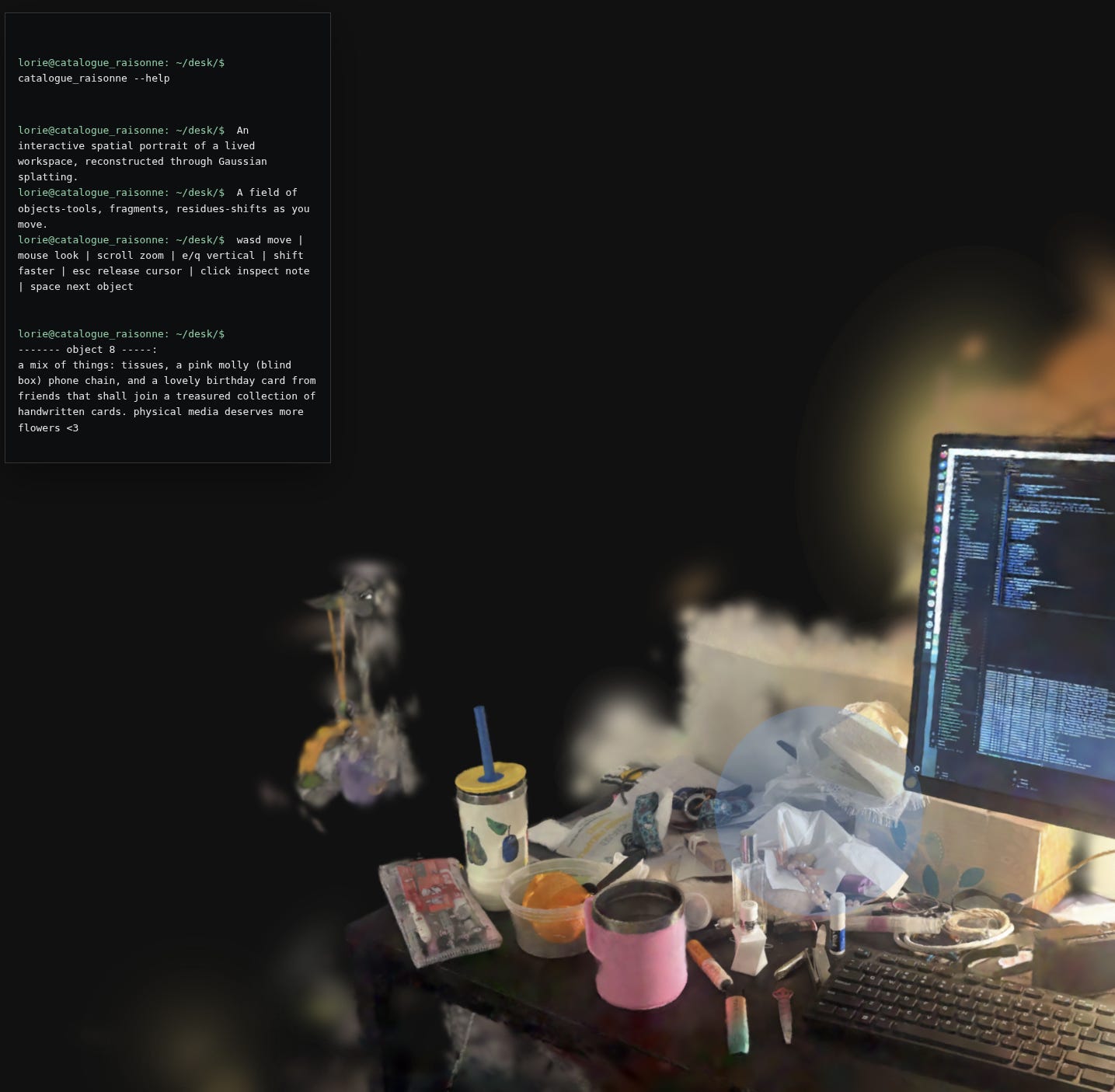
The terminal interface in the top-left corner is intentional. The project lives in a monospace aesthetic — lorie@catalogue_raisonne:~/desk/$ — because I wanted the experience to feel like navigating a filesystem of objects, not browsing a museum. The viewer is structured more like a command line than a gallery.
Clicking an object triggers a typewriter animation that reveals the annotation text associated with that cluster. The effect is slightly slow, slightly imperfect — it feels like something being retrieved from memory rather than looked up in a database.
// index.html — contagion-style typewriter reveal
function typeTerminalHtml(html) {
  const token = ++typewriterToken; terminalOutputEl.innerHTML = ‘’;
  const chars = [...html];
  let index = 0;
  function step() {
    if (token !== typewriterToken) return;
    // cancel if selection changed
    terminalOutputEl.innerHTML = chars.slice(0, index).join(’‘);
    if (index < chars.length) {
      index += 1; window.setTimeout(step, index < 32 ? 10 : 6);
      // faster after initial reveal
    }
  }
  step();
}
Navigation is first-person: WASD to move, mouse to look, scroll to zoom, E/Q for vertical movement, shift to sprint. Pressing space cycles through annotated objects in sequence. The camera can be locked for pointer-lock exploration or unlocked for clicking.
The segment halo — a translucent blue sphere that appears at the selected object’s centroid — scales with the cluster’s Gaussian count, so large objects (the desk surface, the monitor) get proportionally larger halos than small ones (a pen, a cable end).
// halo radius scales with segment size
const gaussianCount = meta.gaussianCount ?? 0;
const radius = Math.max(0.07, Math.min(0.2, 0.07 + gaussianCount / 350000));
selectionHalo.scale.setScalar(radius / 0.085);
The annotation system stores thematic metadata alongside each segment’s label and freeform text. The full theme taxonomy: institution, labor, algorithm, material, translation, routine, memory, accumulation, rest/maintenance, documentation, transit. A theme filtering mode, in which all objects belonging to a selected theme illuminate simultaneously while others dim, is planned but not yet implemented in the public demo.
Future work
The demo currently covers the desk — a tight crop of the bedroom that was the most interesting segmentation challenge and the densest site of practice. Extending it to the full bedroom and studio is the immediate next step.
A few things I want to build:
Contagion interaction. When you click an object, a ripple spreads outward through a proximity graph built from inverse centroid distances: directly adjacent objects activate at high opacity, neighbors-of-neighbors at lower opacity, following an exponential falloff. The effect should feel like heat diffusing through a material network — the room’s relational logic made visible. This is architecturally designed into the annotation data structure; it just needs the front-end interaction layer.
Community annotation. Objects that hold different memories for different people. Tools that have accumulated gradually vs. things that arrived for a specific project. The room as a record of duration and flow of people, not just arrangement.
Sound. Ambient audio associated with different regions — the hum of the computer at the desk, the specific quiet of the studio in the morning. The spatial audio should be spatialized to the 3D positions of the objects that produce it.
Quantitative validation of HPRO floater suppression. I have visual confirmation that floater removal improves segmentation boundaries, but I haven’t run formal PSNR/SSIM comparisons between the pre- and post-suppression splats. That’s next.
Studio capture. The bedroom is done. The studio is where I paint, where there’s more physical mess and less computational infrastructure. It will be a different segmentation challenge — paint tubes, canvases, surfaces with actual texture — and a different interpretive register.
The project is live at https://room.loriechen.com/. The code is available on request. If you end up scanning your own room and running the segmentation pipeline, I’d genuinely like to know what parameters you ended up with for HDBSCAN.